Chapter 2. Basic Ngspice, Xyce and SPICE OPUS simulation

2.1 Introduction

This section describes a number of fundamental methods for launching circuit simulations from the Qucs GUI using the Ngspice, Xyce and SPICE OPUS compatible simulator engines. Spice4qucs includes built-in support for SPICE via a subsystem specifically designed for this purpose. The Ngspice, Xyce and SPICE OPUS simulators are not embedded in Qucs but operate as independent external simulators. Before use they must be installed on the computer operating system that you are running Qucs.

2.2 Supported simulators

Ngspice is a mixed-level/mixed-signal circuit simulator implemented from three open source software packages: SPICE 3f5, Cider 1b1 and XSPICE. Ngspice is one of the most widely used and stable current generation open source SPICE simulators available. It implements the original SPICE3f5 simulation capabilities, including for example, DC, AC, and transient simulation, Fourier-analysis and sensitivity analysis, plus a significant number of extra simulation and device model extensions. Distributed with Ngspice is a data manipulation package called Ngnutmeg. This provides numerical analysis and visualisation routines for post processing Ngspice simulation data. Instructions for installing Ngspice can be found on the Ngspice website at http://ngspice.sourceforge.net/download.html, The Ngspice website also gives free access to all the distribution and development package code sources.

Xyce is an open source, SPICE-compatible, high-performance analogue circuit simulator, capable of solving extremely large circuit problems when installed on large-scale parallel computing platforms. It also supports serial execution on all common desktop platforms, and small-scale parallel execution on Unix-like systems. Xyce for Linux, Microsoft Windows, and MacOS can be downloaded from the official Xyce website at https://xyce.sandia.gov/Xyce. The Xyce parallel circuit simulator running on Linux requires installation of the openMPI libraries. Spice4qucs supports both Xyce-Serial and Xyce-Parallel (not currently available for the Microsoft Windows operating system).

SPICE OPUS is an improved version of SPICE based on the original SPICE 3f5 code with extensions for circuit and device performance optimization and a transient simulation shooting method for large signal steady state AC analysis. SPICE OPUS can be downloaded from its official website at http://www.spiceopus.si/.

Although Ngspice, Xyce and SPICE OPUS are all compatible SPICE simulators they also include extensions to the original SPICE 3f5 netlist syntax which are often incompatible and may not simulate but generate errors. The Qucs Team is aware of this limitation and are attempting to correct such problems as quickly as possible. Please note this may take some time. However, if you do identify a compatibility bug please inform us by sending in a bug report to the Qucs web site (with an example test schematic if possible) describing the problem you have identified.

2.3 General simulation methods

The starting point for understanding how the spice4qucs extensions are built into the Qucs GUI is to study the basic operations needed to simulate Qucs circuit schematics with external simulators. For this purpose consider the simple RCL circuit shown in Figure 2.1.

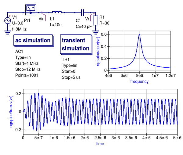
Figure 2.1. A simple RCL test circuit for demonstrating Ngspice, Xyce and SPICE OPUS simulation controlled from Qucs.

This schematic specifies two simulations:

• AC simulation from 4 MHz to 12 MHz.
• Transient simulation from 0 to 5 us;

Make sure the schematic in Figure 2.1 is drawn correctly then simulate it with Qucsator using the sequence Simulation->Simulate, or by pressing key F2. After Qucs finishes the the AC and transient simulations, plot the output data listed below:

• The voltage across R1 resistor in the frequency domain (given by the voltage at the Vr node ),
• The input and output voltage waveforms (the voltages given by the Vin and Vr nodes ) - your plots should be similar to those shown in Figure 2.1,
• The current in the frequency domain (Pr1 current probe ),
• The transient current waveform sensed by the current probe Pr1.

Spice4qucs allows schematic component properties to be defined in the same way as Qucs. Component values and other icon properties are converted automatically into SPICE compatible netlist format. There is no need for manual adaptation by users. However, please note that not all the predefined Qucs components are available for simulation with Ngspice, Xyce or SPICE OPUS. A number of tables provided in later sections of the text list which components can be used with which simulator. Following placement and wiring of components, plus the addition of one or more simulation icons, SPICE simulation is launched using the Qucs menu sequence Simulation -> Simulate or by pressing key F2. An External simulator dialogue then appears. This is illustrated in Figure 2.2.

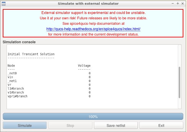
Figure 2.2. External simulator dialogue: where button Simulate launches a circuit simulation, button Stop causes a running simulation to finish; button Save netlist generates, and stores, the netlist of the circuit being simulated and button Exit closes the external simulator dialogue.

If the Ngspice, Xyce or SPICE OPUS installation directories are not included in the operating system shell $PATH statement the location of their executable code must be registered with spice4qucs before Ngspice Xyce or SPICE OPUS simulations will work. This step is necessary for all the operating systems used to run spice4qucs. To register external circuit simulator installation directories spice4qucs users need to launch the Select default simulator, from the Simulate dialogue. The resulting Setup simulators executable simulator location dialogue is illustrated in Figure 2.3. Using this dialogue enter the absolute address of the Ngspice, Xyce or SPICE OPUS executable program code from the keyboard or by pressing the appropriate Open File Select button.. In the case of the Xyce Parallel simulator the number of processors installed in your computer system, must also be entered from the keyboard or selected using the dialogue up-down arrow controls.

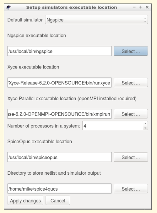
Figure 2.3. Setup simulator executable locations dialogue.

Please note the Xyce parallel command line for binary Xyce-Parallel package has the following format:

<Path_to_xyce_executable>/xmpirun -np %p

Where spice4qucs substitutes the number of processors for the %p wildcard entry.

Also please note that “user builds” of Xyce-Parallel have no xmpirun script, implying that the full script must be completed by users during the external simulators set up process, for example if opeMPI is installed in directory /usr/bin and Xyce-Parallel installed in /usr/local/Xyce_Parallel the command line will be:

/usr/bin/mpirun -np %p /usr/local/Xyce_Parallel/bin/Xyce

Spice4qucs users can also define a directory where temporary simulator data and netlists are stored: this simulator working directory is by default assumed to be at $HOME/.qucs/spice4qucs.

To simulate a Qucs schematic with the Ngspice simulator, select simulator Ngspice and press the Simulate button shown in Figure 2.2. During simulation Ngspice produces a simulation log. This is displayed in the External simulator dialog window, see Figure 2.4. The Qucs Log text is also saved at Qucs system Log location $HOME/.qucs/log.txt. The Log text can be viewed and using the drop down menue sequence Simulation->Show last messages (or by pressing key F5). If the Ngspice simulation fails, any errors reported by Ngspice during simulation are listed in simulation Log window. Similarly, a successful completion of a Qucs/Ngspice simulation is reported.

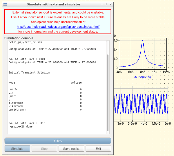
Figure 2.4. A section of an Ngspice execution Log displayed in the Simulate with an external simulator dialogue window.

An novel feature introduced by spice4qucs is its ability to generate and save SPICE netlist files from the information contained in a Qucs schematic. To save the SPICE netlist file for the current simulation press the Save netlist button shown in Figure 2.2. This process causes a SPICE netlist to be saved as file “netlist.cir” in the ~/.qucs/spice4qucs directory. Here is the generated netlist for the RCL test example:

* Qucs 0.0.19  /home/vvk/qucs/examples/ngspice/RCL.sch
V1 _net0 0 DC 0 SIN(0 0.6 7.5MEG 0 0) AC 0.6
VPr1 _net0 vIn DC 0 AC 0
L1 vIn _net1  10U 
R1 0 vR  30
C1 _net1 vR  40P 
.control
set filetype=ascii
AC LIN 1000 4MEG 12MEG 
write RCL_ac.txt VPr1#branch v(vIn) v(vR) 
destroy all
TRAN 4.97512e-09 1e-06 0 
write RCL_tran.txt VPr1#branch v(vIn) v(vR) 
destroy all
exit
.endc
.END

The simulation sequence introduced in the previous sections of the spice4qucs-help text also applies to the Xyce and SPICE OPUS simulators. However, the information displayed in the simulation log is likely to be different for different simulators and indeed operating systems.

After an Ngspice, Xyce or SPICE OPUS simulation has successfully completed close the External simulation dialogue by pressing the “Exit” button. The simulation data generated by a spice4qucs simulation is available for plotting using the normal Qucs visualisation routines: either drag a diagram icon, or table icon, onto the current Qucs schematic window or onto the associated Qucs display page. After a diagram or table is placed a Diagram properties dialog appears. On selecting the dataset for the current simulation the simulation output quantities become available for plotting or tabulating in a similar fashion to standard Qucs.

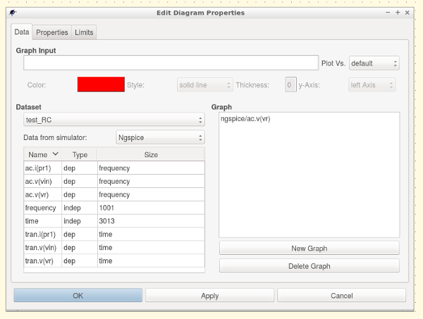
Figure 2.5. Diagram properties dialogue, listing the selected simulator and the available simulation data names.

Ngspice, Xyce and SPICE OPUS simulation data output is in raw-binary SPICE 3f5 output format. Qucs converts the SPICE 3f5 style data into a Qucs dataset using routines provided in the spice4qucs Qucs subsystem. Results from different types of simulation, for example SPICE AC and TRAN, are combined into a single Qucs dataset. Qucs adds an appropriate suffix to each simulator dataset name in order to avoid name clashes and mixing up results from different types of simulation. In the RCL test example the Qucs schematic is named RCL.sch. Qucs qucsator simulation, Ngspice, Xyce and SPICE OPUS simulations result in three different datasets:

• RCL.dat — for Qucsator;
• RCL.dat.ngspice — for Ngspice;
• RCL.dat.xyce — for Xyce;
• RCL.dat.spopus — for SPICE OPUS;

All four datasets have an extension dat to signify that each set contains Qucs data for post simulation visualisation. The Ngspice, Xyce and SPICE OPUS datasets include second a extension to the file name to identify the name of the external Qucs simulator.

The Dataset selector (see Figure 2.5) shows only the base names of a dataset (for example test_RC). Users must also select the appropriate simulator from the simulator name selector drop-down list. This drop-down only gives existing simulator datasets which prevents users from selecting non-existent datasets by mistake.

Following the selection of a specific data set users must select the variables that are to be plotted. Spice4qucs preserves SPICE notation for node voltage names and current probe names. SPICE names are assumed to be case insensitive by spice4qucs, for example

• v(out) — Voltage at node out;
• i(Pr1) — Current recorded by current probe Pr1;

The Qucs spice4qucs extension also adds a simulation-dependent prefix to each variable name in order to differentiate output variables from different SPICE simulations, for example ac. for AC simulation, tran. for transient simulation, and dc. for DC-sweep.

There are also individual prefixes for each simulator:

• ngspice/ — Ngspice simulator prefix;
• xyce/ — Xyce simulator prefix;
• spopus/ — SPICE OPUS prefix;

Hence for example, the full name of variable from an Ngspice simulation could be ngspice/v(out) This naming system helps to avoid dataset name conflicts.

Individual items for plotting are selected by double clicking on a name in the variable list. As an example when double clicking on ac.i(pr1) its name is copied by Qucs into the right-hand plotting window. Like standard Qucs one or more variable items may be selected for plotting on the same 2D or 3D graph. Finally pressing the Apply button shown at the bottom of Figure 2.5. causes the selected variable items to be plotted. The plotted simulation results for the external Ngspice AC simulation of the RCL test circuit are shown in Figure 2.6.

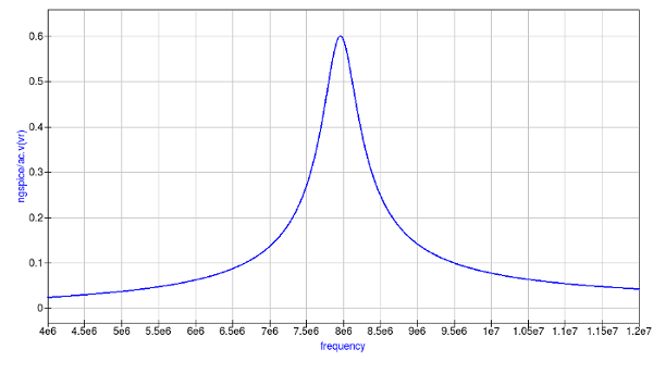
Figure 2.6. External SPICE AC simulation magnitude response for the current flowing in RCL circuit with a series resonant peak of roughly 8 MHz .

Plotting the transient simulation data for the RCL test example follows the same procedure as the sequence described for the AC simulation except that in the transient plot variables with tran in their name are selected, see Figure 2.7.

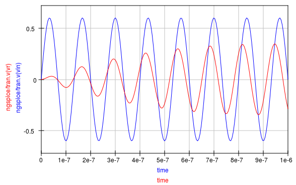
Figure 2.7. Transient simulation voltage waveforms at the input and output nodes of the RCL circuit.

A similar proceedure is adopted for plotting simulation data generated with the Xyce and SPICE OPUS simulators. Readers should make sure they can simulate the example RCL circuit with both Xyce and SPICE opus, then plot the resulting simulation data. More advanced techniques for post processing, plotting and undertaking a range of different visualization processes using Qucs and Octave are outlined in chapter 7.

2.4 Variable names

As part of the spice4qucs extensions Ngspice and Xyce simulation variable names are converted from Qucs notation to SPICE notation and vica versa. Table 2.1 shows the correspondence between the two notations.

Table 2.1 Qucs and SPICE variable equivalences

Variable type	Qucs display notation	Spice display notation
DC node voltage	Node.V	V(node)
AC node voltage	Node.v	ac.v(node)
TRAN node voltage	Node.Vt	tran.v(node)
HB node voltage	Node.Vb	hb.v(node)
DC probe current	Pr1.I	i(pr1)
AC probe current	Pr1.i	ac.i(pr1)
TRAN probe current	Pr1.It	tran.i(pr1)

Also variable prefixes used to designate data from different simulators (Table 2.2)

Table 2.2 Qucs and SPICE variable name prefixes

Prefix	Explanation
Node.Vt	Qucs simulation, default dataset
dataset:Node.Vt	Qucs simulation, external dataset
ngspice/tran.v(node)	Ngspice simulation, default dataset
ngspice/dataset:tran.v(node)	Ngspice simulation, external dataset
xyce/tran.v(node)	Xyce simulation, default dataset
xyce/dataset:tran.v(node)	Xyce simulation, external dataset
spopus/tran.v(node)	SPICE OPUS simulation, default dataset
spopus/dataset:tran.v(node)	SPICE OPUS simulation, external dataset

2.5 DC simulation

Conventional SPICE 3f5 simulation commands OP and DC are not implemented by Qucs or indeed by spice4qucs. Instead more convenient versions of these simulation commands are implemented. These alternative forms of non-linear steady state DC circuit analysis are linked directly to circuit schematic capture, making them easy to use. Moreover, they provide spice4qucs users with a power full diagnostic and analysis tools for investigating basic circuit operation. The circuit shown in Figure 2.8 represents a simple resistive network with single voltage and current 1 V and 1 A sources respectively. Pressing key “F8” instigates a DC analysis and adds the DC node voltages, probe voltages and probe currents to the current schematic. This feature provides a practical method for scanning a circuit to see if the DC bias values are of the correct order of magnitude. The calculation of DC bias values via the F8 key applies to all the circuit simulators controlled by spice4qucs. Schematics which include the spice4qucs DC icon do not however, list a similar set of voltage and currents in the *Simulate with an external Simulator” dialogue window. A DC voltage and current list is output when a schematic includes a transient simulation icon, see Figure 2.9.

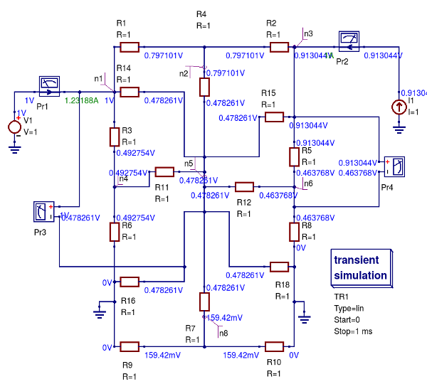
Figure 2.8 A simple linear resistive electrical network driven by single DC voltage and current sources: DC node voltages (V) and voltage probe values (V) are illustrated in blue and current probe values (A) in green.

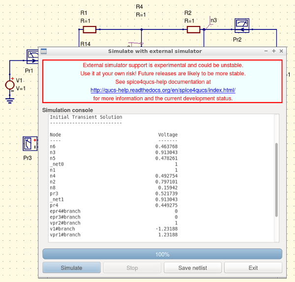
Figure 2.9 A screen dump showing transient simulation initial DC simulation voltage and current values in (V) and (A) respectively for the resistive circuit given in Figure 2.8: NOTE that the voltage and current variable names are output in SPICE style syntax.

Qucs does not define a separate analysis type which is equivalent to the original SPICE 2g6 “DC sweep” simulation or the extended SPICE 3f5 version which allows current and voltage source scans plus resistor value scans. In contrast to SPICE the Qucs equivalent “DC sweep” is just a specific case of the more general Qucs Parameter sweep capability. To emulate the original SPICE DC sweep` spice4qucs use a combination of Qucs DC simulation plus the Parameter sweep of an independent DC voltage or DC current source or of a resistor numerical value; when the spice4qucs Spice netlist builder finds these two linked types of simulation it synthesises them into a DC SPICE netlist entry. This procedure is demonstrated in Figure 2.10. where the test circuit consists of a diode DC bias network connected as a test bench for simulating the non-linear DC current-voltage characteristic of a 1N4148 diode. This example can be found in the Qucs examples directory tree listed as examples\ngspice\diode.sch .

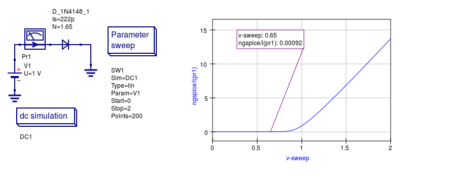
Figure 2.10. Test circuit and simulated DC current-voltage characteristics for a 1N4148 silicon diode.

PLease note the following differences between SPICE and Qucs DC-sweep simulation:

• Specify a sweep source name or a resistor name NOT a source or resistor value; for example in Figure 2.10 V1.
• SPICE model parameters can be swept using the notation Device.Param, for example T1.Bf to sweep the Bf parameter of transistor T1.

2.6 AC simulation

Small signal AC simulation is fully supported by the spice4qucs subsystem. It doesn’t require any special adaptation. Just simple place the AC simulation component icon on a schematic and execute an Ngspice, Xyce or SPICE OPUS simulation. Variable name conversions are listed in Table 2.1. The Qucs spice4qucs dataset builder adds the ac. prefix to all variables generated by an AC simulation.

Ngspice, Xyce and SPICE OPUS small signal frequency domain AC simulations use linear, decade or octave frequency scales. Adaptive frequency steps are not implemented.

2.7 TRANsient simulation

Transient simulation is also fully supported by the spice4qucs subsystem. Just place the Transient simulation component icon on a schematic and simulate it. There is a difference between the way the qucsator, Ngspice, Xyce and SPICE OPUS simulators implement transient simulation time steps.

Qucsator always uses a fixed time step. Ngspice, Xyce and SPICE OPUS use adaptive time steps. The number of simulation points output during a simulation will only be approximately equal to the number of simulation points specified in a Transient simulation properties list. For example, in an example test circuit 200 time points are specified on the schematic. However, due to the fact that the SPICE simulators use adaptive time steps, Ngspice employs 213 simulation points, and Xyce employs 799 time points. This difference should be taken into account during simulation data post processing and when comparing simulation results.

2.8 Other forms of simulation

In contrast to SPICE 3f5, the parameter sweep facility found in Qucs has also been implemented with Ngspice, Xyce and SPICE OPUS where the parameter sweep setup and control is organized by spice4qucs. The details of how this Parameter sweep feature works is the topic of section 5.8.

As well as the fundamental DC, AC and transient simulation types, Ngspice, Xyce and SPICE OPUS also support the additional forms of simulation listed in Table 2.3.

Table 2.3 Spice4qucs simulation types additional to DC, AC and TRAN

Simulation Type	Ngspice	Xyce	SPICE OPUS	See section
Fourier	X	X	X	5.1
Distortion	X		X	5.2
Noise	X	X	X	5.3
Pole-zero	X		X	5.4
Sensitivity	X	X	X	5.5
Harmonic Balance		X		13.5
Tran shooting method			X	13.7
Custom simulation	X		X	8.0

Fourier, distortion pole-zero circuit simulation require special GUI icons. These can be found in the Qucs Spice simulations group. In contrast sensitivity, the SPICE OPUS tran shooting method is accessed by spice4qucs via the Custom simulation technique, see section 8.0.

2.9 Spice4qucs circuit simulation components

Qucs is released with a good selection of passive and active component models. This selection includes both fundamental circuit components, like R, C and L and collections of specific components for a given circuit design sector, like the RF microstrip component models. All the original Qucs component and device models were written to work with Qucs and there is NO Guarantee that they will be work with Ngspice, Xyce or SPICE OPUS. For circuit simulation packages which take advantage of simulation multi-engines this can be a serious problem, particularly for the less experienced user. To help reduce problems to a minimum, spice4qucs uses a policy of “blacklisting” those models which do not work with the chosen circuit simulation engine. This policy works in the following way:- when a specific simulator is chosen by a Qucs spice4qucs user, on running the chosen simulator, ONLY those models which work with the selected simulator become available for drawing circuit schematics and simulation. The same approach applies to the components held in the spice4qucs libraries.

2.10 More basic simulation examples

2.10.1 DC Example 1: Calculating circuit input resistance and power dissipation in a resistor.

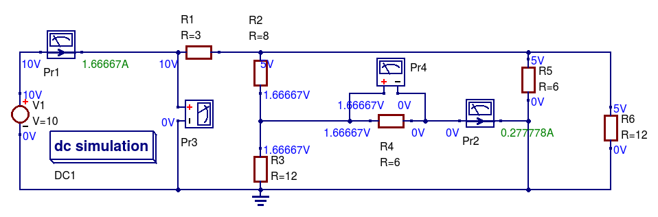
Figure 2.11 DC resistive test network.

• Draw the circuit diagram shown in Figure 2.11,
• Select simulator Ngspice,
• Press key F8
• Determine DC Rin = V(Pr3)/I(Pr1) = 10/1.66667 = 6 Ohm,
• Determine the power dissipated in R4 = V(Pr4)*I(Pr2) = 1.66667*0.277778 = 0.463 W.

2.10.2 DC Example 2: Variation of power dissipation with varying DC input voltage.

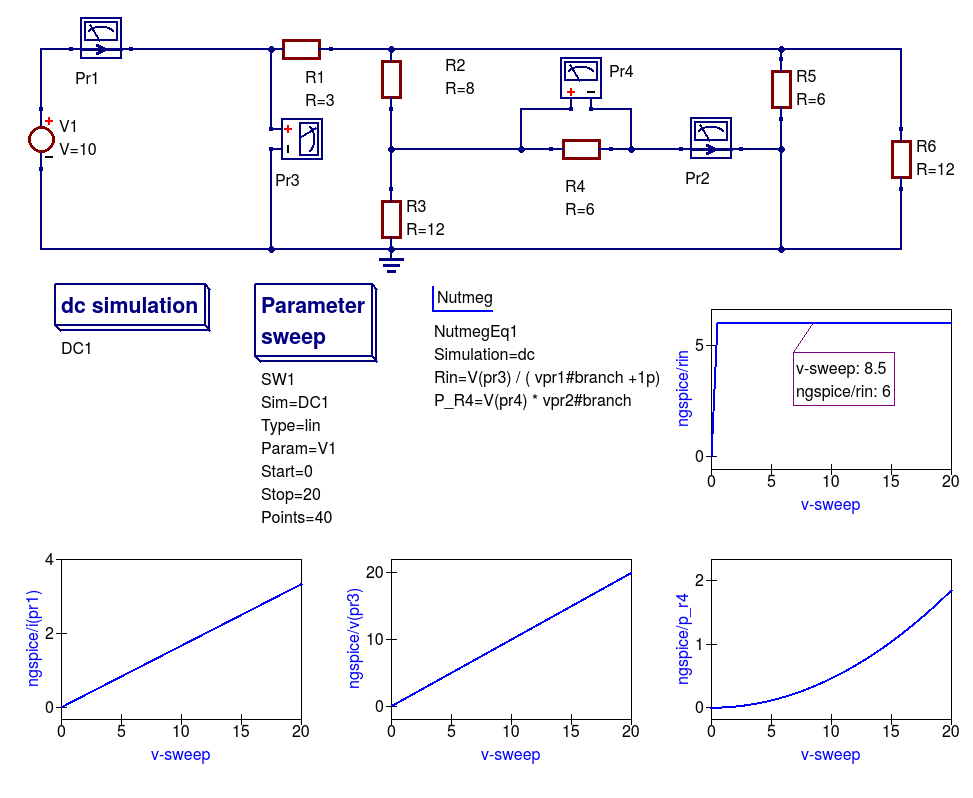
Figure 2.12 DC example 1 with varying DC input voltage: demonstrating the use of a DC sweep simulation.

• Draw the circuit diagram shown in Figure 2.11,
• Select simulator Ngspice,
• Add the dc simulation, Parameter sweep and Nutmeg component icons to the drawn schematic,
• Complete the Parameter sweep and Nutmeg component data entries so that they are the same as given in Figure 2.11,
• Press the F2 to simulate the circuit,
• Plot the graphs illustrated in Figure 2.11,
• Check that your results are the same - if not or the simulation fails check your schematic for errors and re-simulate.

Notes:

• Current probe values are represented by the SPICE 3f5 notation: vpr1#branch and vpr2#branch.
• There is a discontinuity in Rin when the vpr1#branch current is zero Amperes; hence the need for the dummy 1pA in the Nutmeg equation for Rin.

back to the top